The analysis of the properties of products and their sales in the respective outlets helps a brand to skyrocket its sales and ensure customer satisfaction.

In this article, I have explored the Big Mart sales problem and have performed the analysis of various products and outlets using SQL.

About the Dataset:

I have used 100 rows of the following dataset:

https://www.kaggle.com/datasets/shivan118/big-mart-sales-prediction-datasets?select=train.csv

This data has been collected by the data scientists at BigMart from the sales of 2013 for 1559 products, spread across 10 stores in multiple cities.

The columns are:

1. Item_Identifier: product ID

2. Item_Weight: weight of the product

3. Item_Fat_Content: fat content(low fat or regular fat) of the product

4. Item_Visibility: The total display area allotted to the product in percentage

5. Item_Type: category of the product

6. Item_MRP: MRP of the product

7. Outlet_Identifier: unique ID of the outlet

8. Outlet_Establishment_Year: year of establishment of the outlet

9. Outlet_Size: the size of the outlet

10. Outlet_Location_Type: type of city where the outlet is located( tier 1/tier 2/tier 3)

11. Outlet_Type: type of outlet (supermarket/grocery store)

12. Item_Outlet_Sales: sales of the product in a particular outlet

These rows and columns have been stored in a table that I have named 'bigmart'.

Data Cleaning:

Checking for Null Values in Outlet_Size attribute:

select count(*),Outlet_Size from bigmart group by Outlet_Size;

The output is:

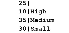
As observed from the above result, there are 25 NULL values in Outlet_Size. Since Medium sized outlet is the most popular type, we replace the null values of Outlet_Size with "Medium" in the following manner:

update bigmart set Outlet_Size='Medium' where Outlet_Size is NULL;

To check if the updates have been reflected or not, the next query is run:

select count(*),Outlet_Size from bigmart group by Outlet_Size;

The output is:

Checking for Null values in Item_Weight Attribute:

select count(*) from bigmart where Item_Weight is NULL;

The output is 19.

To fill up the null values in the Item_Weight attribute, the average of Item_Weight is calculated and put in place of the null values as follows:

select avg(Item_Weight) from bigmart;

The output is 13.127037037037.

Now, the Item_Weight's null values are replaced with the above value in the manner given below:

update bigmart set Item_Weight=13.127037037037 where Item_Weight is NULL;

To check if the changes have been reflected in the table or not, the next query is run:

select * from bigmart where Item_Weight is NULL;

No rows are displayed. Hence, the null values have been successfully tackled.

Checking the type of values taken by Item_Fat_Content attribute:

select distinct Item_Fat_Content from bigmart;

The result is:

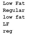
Low Fat, low fat and LF mean the same thing. Also, Regular and reg hold the same meaning. Hence the values are updated as follows:

update bigmart set Item_Fat_Content='low fat' where Item_Fat_Content='LF' or Item_Fat_Content='Low Fat';
update bigmart set Item_Fat_Content='regular' where Item_Fat_Content='reg' or Item_Fat_Content='Regular';

To check if the changes have been successfully implemented or not, the next query is run:

select distinct Item_Fat_Content from bigmart;

The output is:

Analyzing the Fat Content Attribute:

Checking the average MRP of items with respect to Fat Content:

select avg(Item_MRP),Item_Fat_Content from bigmart group by Item_Fat_Content order by avg(Item_MRP) desc;

The output is:

Low-fat content items have a higher average MRP than regular fat-content items.

Finding the average sales of items in Outlets with respect to Fat Content:

select avg(Item_Outlet_Sales),Item_Fat_Content from bigmart group by Item_Fat_Content order by avg(Item_Outlet_Sales) desc;

The output is:

Low-fat items have recorded the highest average amount of sales.

Determining the average visibility provided to items with respect to Fat Content:

select avg(Item_Visibility),Item_Fat_Content from bigmart group by Item_Fat_Content order by avg(Item_Visibility) desc;

The output is:

Regular fat-content items are provided with more visibility as compared to low-fat content items.

Analyzing the Item_Type attribute:

Checking the average MRP of items with respect to Item_Type:

select avg(Item_MRP),Item_Type from bigmart group by Item_Type order by avg(Item_MRP) desc;

The output is:

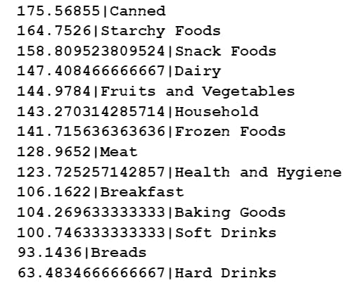
Canned Food items have the highest average MRP whereas Hard Drinks have the lowest MRP.

Finding the average sales of items in Outlets with respect to Item_Type:

select avg(Item_Outlet_Sales),Item_Type from bigmart group by Item_Type order by avg(Item_Outlet_Sales) desc;

The result is:

Starchy Foods are in high demand as average sales are higher than the rest of the types. Hard Drinks are the lowest in demand since average sales are the lowest among all the types.

Determining the average visibility provided to items with respect to Item_Type:

select avg(Item_Visibility),Item_Type from bigmart group by Item_Type order by avg(Item_Visibility) desc;

The output is:

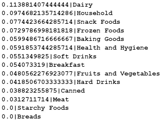
Dairy and Household products are given the highest amount of visibility whereas starchy foods and breads have the lowest amount of visibility.

Finding the total sales of all outlets:

select sum(Item_Outlet_Sales),Outlet_Identifier from bigmart group by Outlet_Identifier order by sum(Item_Outlet_Sales) desc;

The output is:

OUT046 has the highest amount of sales whereas OUT010 has the lowest amount of sales.

Finding the average sales with respect to Outlet_Type:

select avg(Item_Outlet_Sales),Outlet_Type from bigmart group by Outlet_Type order by avg(Item_Outlet_Sales) desc;

The output is:

Supermarket Type2 have the highest amount of average sales whereas grocery store has the lowest amount of sales on average.

Determining the average sales with respect to Outlet_Size:

select avg(Item_Outlet_Sales),Outlet_Size from bigmart group by Outlet_Size order by avg(Item_Outlet_Sales) desc;

The output is:

Medium-sized outlets have the highest recorded average sales whereas High (or large) sized outlets have lesser sales on average.

Checking the average sales with respect to Outlet_Location_Type:

select avg(Item_Outlet_Sales),Outlet_Location_Type from bigmart group by Outlet_Location_Type order by avg(Item_Outlet_Sales) desc;

The output is:

Tier 2 cities have recorded the highest average sales whereas Tier 1 cities have recorded the least average sales.

Determining the average sales with respect to Outlet_Establishment_Year:

select avg(Item_Outlet_Sales),Outlet_Establishment_Year from bigmart group by Outlet_Establishment_Year order by avg(Item_Outlet_Sales) desc;

The output is:

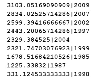
The outlets established in 2009 and 2007 have recorded the highest average sales whereas the outlets established in 1998 have the lowest sales on average.

---

Found this article interesting? Give it a like and share it with your friends!

Follow Analytics With Amruha for more updates: https://www.instagram.com/analyticswithamruha/?next=%2F

#data #datascience #dataanalytics #dataanalysis #analytics #analysis #bigmart